Chapter 3 Descriptive Analysis
See Appendix section 5.2 for the R code used in this chapter.
Note: for conciseness, the following examples will only show results for two of the four gendered aspects of health items from the SGBA-5 (gender identity, and gender roles)
3.1 Visualize Distribution of SGBA-5 Responses
3.1.1 Biological Sex Item
In plot 3.1 we see that there are more participants who report their biological sex as assigned as female at birth (n=18) than males (n=12).
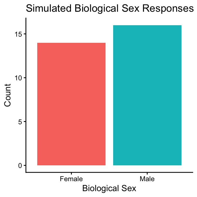
Figure 3.1: Barplot of Biological Sex Responses
3.1.2 Gendered Aspect of Health Items
Looking at the density plots for gender identity and gender role (figure 3.2), we see that while both variables are bimodal, the gender identity responses is more strongly bimodal with one peak closer to the feminine side of the feminine-masculine continuum and one peak closer to masculine end of that continuum. Further, we can also see that in general, participants reported their gender identity and roles as being more feminine, again with the gender identity responses showing this trend more strongly than the gender role responses.
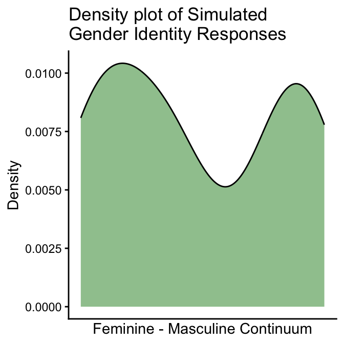
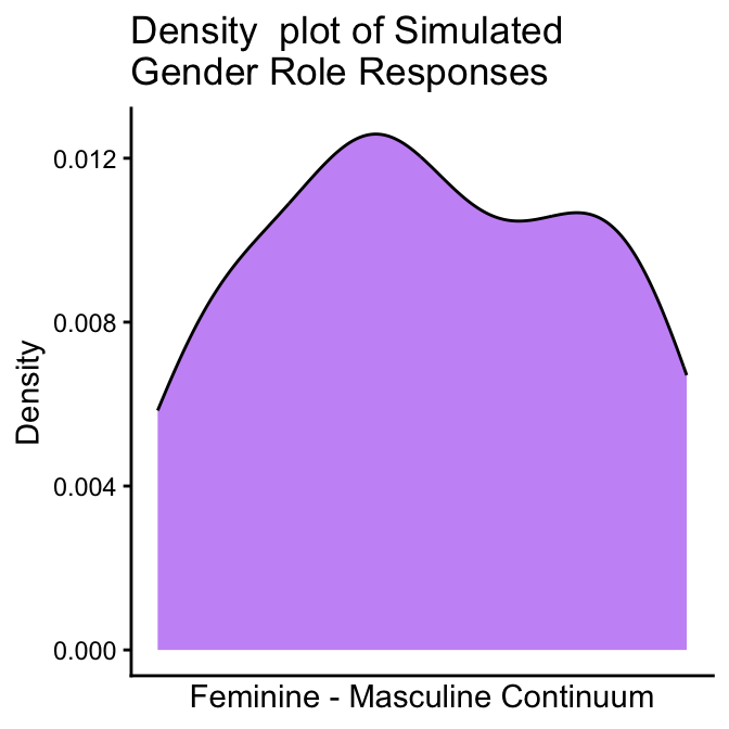
Figure 3.2: Density plots of Gender Identity and Roles
Presently, there is no clear consensus on how to present descriptive statistics of bimodal variables in health research. Reporting the mean(sd) or median(IQR) of a variable does not clearly communicate that there is more than one peak in a bimodal variable’s distribution.
When taken alongside the SGBA-5’s assumption that the feminine-masculine continuum doesn’t have a true 0 value, it is our suggestion that:
If researchers decide to report a descriptive statistic for a bimodally distributed variable, they should report a nominal description of the variable’s distriubtion skew.
For example, if a gendered aspect of health item from the SGBA-5 demonstrates a bimodal distribution, the variable’s skew can be described along the feminine-masculine continuum instead of reporting the numerical average alone.
To be able to describe the skew of one of the gender variables, the authors suggest calculating the variable’s mean score along the feminine-masculine continuum and then reporting the skew using the suggested nominal classification guide seen in Table 3.1.
Please note that these suggested classification guidelines are arbitrary and may not be appropriate in all circumstances.
| Mean | Interpretation |
|---|---|
| >70 | “Skews masculine” |
| 55 to 70 | “More masculine than feminine” |
| 45 to 55 | “Not strongly skewed” |
| 30 to 45 | “More feminine than masculine” |
| <30 | “Skews feminine” |
Note: This table assumes you have recorded the gendered aspects of health items as 0 being the most feminine score and 100 being the most masculine score.
For the simulated dataset represented in the density plots above, the mean score for the gender identity item was 50.2 and 46.8 for the gender role item. This means that when reporting descriptive statistics on the simulated sample we could report that: “The simulated sample was not strongly skewed on a feminine to masculine continuum for either the gender identity or gender role measures from the SGBA-5”.
3.2 Descriptive Table of SGBA-5 Responses
Taking all these together, an example of a sample characteristics table of the SGBA-5 items in the simulated dataset could be presented as has been displayed in Table 3.2
| SGBA Item | Sample (n = 30) |
|---|---|
| Biological Sex (n(%)) | |
| Female | 14(47%) |
| Intersex | NA |
| Male | 16(53%) |
| Gendered Aspect of Health (skew) | |
| Gender Identity | Not strongly skewed |
| Gendered Roles | Not strongly skewed |
See Appendix section 5.2 for the R code used in this chapter.